Simple FWI Example

In this section we see application of PyFWI for performin FWI. First, forward modeling is shown and then we estimate a model of subsurface using FWI.

1. Forward modeling

In this simple example, we use PyFWI to do forward modeling. So, we need to first import the following packages amd modulus.

import matplotlib.pyplot as plt
import numpy as np

import PyFWI.wave_propagation as wave
import PyFWI.acquisition as acq
import PyFWI.seiplot as splt
import PyFWI.model_dataset as md
import PyFWI.fwi_tools as tools
import PyFWI.processing as process
from PyFWI.fwi import FWI

A simple model can be created by using model_dataset module as

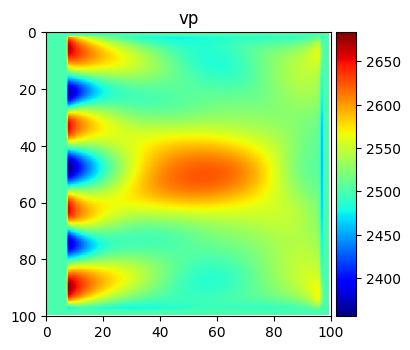
Model = md.ModelGenerator('louboutin')
model = Model()

im = splt.earth_model(model, cmap='coolwarm')

Then we need to create an input dictionary as follow

model_shape = model[[*model][0]].shape

inpa = {
    'ns': 4,  # Number of sources
    'sdo': 4,  # Order of FD
    'fdom': 15,  # Central frequency of source
    'dh': 7,  # Spatial sampling rate
    'dt': 0.004,  # Temporal sampling rate
    'acq_type': 0,  # Type of acquisition (0: crosswell, 1: surface, 2: both)
    't': 0.6,  # Length of operation
    'npml': 20,  # Number of PML
    'pmlR': 1e-5,  # Coefficient for PML (No need to change)
    'pml_dir': 2,  # type of boundary layer
}

seisout = 0 # Type of output 0: Pressure

inpa['rec_dis'] =  1 * inpa['dh']  # Define the receivers' distance

Now, we obtain the location of sources and receivers based on specified parameters.

offsetx = inpa['dh'] * model_shape[1]
depth = inpa['dh'] * model_shape[0]

src_loc, rec_loc, n_surface_rec, n_well_rec = acq.acq_parameters(inpa['ns'],
                                                                 inpa['rec_dis'],
                                                                 offsetx,
                                                                 depth,
                                                                 inpa['dh'],
                                                                 inpa['sdo'],
                                                                 acq_type=inpa['acq_type'])
# src_loc[:, 1] -= 5 * inpa['dh']

# Create the source
src = acq.Source(src_loc, inpa['dh'], inpa['dt'])
src.Ricker(inpa['fdom'])

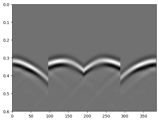
Finally, we can have the forward modelling as

# Create the wave object
W = wave.WavePropagator(inpa, src, rec_loc, model_shape,
                        n_well_rec=n_well_rec,
                        components=seisout, chpr=0)

# Call the forward modelling
d_obs = W.forward_modeling(model, show=False)  # show=True can show the propagation of the wave

plt.imshow(d_obs["taux"], cmap='gray',
           aspect="auto", extent=[0, d_obs["taux"].shape[1], inpa['t'], 0])

<matplotlib.image.AxesImage at 0x15144c760>

2. FWI

To perform FWI, we need the observed data and an initial model.

Note: For better visualization and avoiding crosstalk, I compute the gradient in acoustic media.

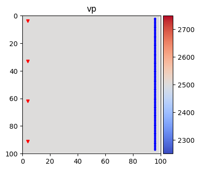
Here is a homogeneous initial model.

m0 = Model(smoothing=1)
m0['vs'] *= 0.0
m0['rho'] = np.ones_like(model['rho'])

fig = splt.earth_model(m0, ['vp'], cmap='coolwarm')

fig.axes[0].plot(src_loc[:,0]//inpa["dh"],
                 src_loc[:,1]//inpa["dh"], "rv", markersize=5)

fig.axes[0].plot(rec_loc[:,0]//inpa["dh"],
                 rec_loc[:,1]//inpa["dh"], "b*", markersize=3)

[<matplotlib.lines.Line2D at 0x158434ee0>]

Now, we can create a FWI object,

fwi = FWI(d_obs, inpa, src, rec_loc, model_shape,
          components=seisout, chpr=20, n_well_rec=n_well_rec)

and call it by providing the initial model m0, observed data d_obs, optimization method method, desired frequencies for inversion, number of iterations for each frequency, number of parameters for inversion n_params, index of the first parameter k_0, and index of the last parameter k_end. For example, if we have an elastic model, but we want to only invert for P-wave velocity, these parameters should be defined as

n_params = 1
k_0 = 1
k_end = 2

If we want to invert for P-wave velocity and then \(V_S\), these parameters should be defined as

n_params = 1
k_0 = 1
k_end = 3

and for simultaneously inverting for these two parameters, we define these parameters as

n_params = 2
k_0 = 1
k_end = 3

Let’s call the FWI object,

m_est, _ = fwi(m0, method="lbfgs",
                 freqs=[25, 45], iter=[2, 2],
                 n_params=1, k_0=1, k_end=2)

# Time to plot the results
fig = splt.earth_model(m_est, ['vp'], cmap='jet')